Excel: Two Stacked, One Clustered Column

Problem: I need to create two stacked columns clustered with a third column.

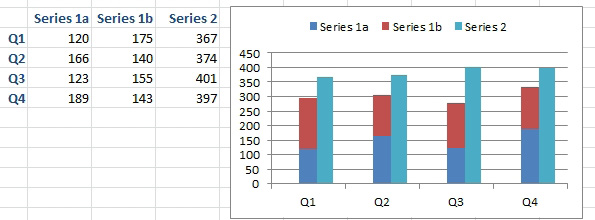
1. This is harder than it looks.

   Strategy: This chart uses two rogue series and a hidden secondary axis. Follow these steps carefully.

   1. Add two blank series between Series 1b and Series 2. Fill with zeroes.

   

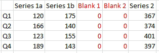
2. Two extra series.
   2. Create a stacked column chart from all five series.
   3. If you are plotting quarters, Excel will put the wrong data along the horizontal axis. Click the Switch Row/Column icon to move the Series 1a, Series 1b, and so on to the legend.
   4. Go to the Layout tab in the ribbon. Use the leftmost dropdown to choose Series 2.
   5. Click Format Selection to open the Format Dialog box.
   6. Choose Secondary Axis. Don't close the Format dialog box.
   7. Go back to the dropdown and choose Series Blank 1.
   8. In the Format dialog box, choose Secondary Axis.
   9. Go back to the dropdown and choose Series Blank 2.
   10. In the Format dialog box, choose Secondary Axis.
   11. Go back to the dropdown and choose Series 2.
   12. Go to the Design tab of the ribbon. Choose Change Chart Type. Choose the first column chart, known as a Clustered Column Chart. This changes all three of the series that use the secondary axis.

   At this point, you finally have something that looks almost correct. There are still several things to fix:

   • The left vertical axis is using a different scale than the first.
   • The stacked column is wider than the clustered column.
   • There are two extra entries in the legend.
   • You really don't need to show the secondary axis once you make them have the same scale.

   

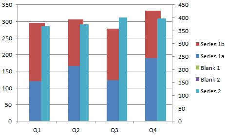
3. You are starting to get close.

   By the way, those two extra blank series are there to move Series 2 to the right. If you entered 100 and 200 in those series, you would see how they are pushing Series 2 over to the right of the stacked column.

   

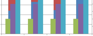
4. Here, the two blank series are moving Series 2 to the right.

   The remaining steps assume the Format dialog box is still open.

   13. Click on the right vertical axis. In the Format dialog, change the first three settings from Auto to Fixed. Make a note of the settings in those three boxes.
   14. Click on the left vertical axis. Make six changes in the Format dialog box. Change the first three settings from Auto to Manual. Click in the box next to manual. Type the same values from step 13 into the boxes next to manual. This will make sure that both axis have the same scale.
   15. Click on one of the stacked series to select it. In the Format dialog box, change the gap width to 300%. This will make the stacked column less wide and about the same size as the third column.
   16. In the legend, click once on Blank 1, then do a second single click on Blank 1 to select only that item in the legend. Press Delete to Delete that entry.
   17. Do two single clicks on Blank 2 in the legend. Press Delete.
   18. In the Layout tab, choose Legend, Show Legend at Top.
   19. Click on the right vertical axis. Press Delete.

   This whole set of steps is demonstrated in Learn Excel Podcast Episode 1091.

   Gotcha: This only works with one stacked column and one non-stacked column. If you need both columns to be stacked, it will not work. Jon Peltier sells a cool utility to solve this.