
Problem: I want to manually format a pivot table. Can I select all the row subtotals? For example, select the region totals in rows 8, 12, and 16.
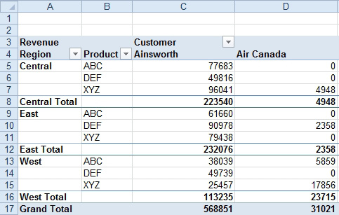
- Select row subtotals.
Strategy: A clever mouse trick will allow you to select similar rows in a pivot table. Follow these steps:
- Select one cell in the pivot table. On the Design tab, choose Report Layout, Show in Tabular Form.
- Hover the mouse over cell A8. This is the Central region total. Slowly move the mouse toward the left edge of the cell. Eventually, the cell pointer changes to a black arrow that points to the right. When this cell pointer appears, click the mouse. Excel will now select all the subtotal rows.
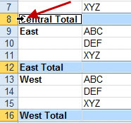
- One click select all subtotal rows.
- Using the formatting icons on the Home tab of the ribbon, assign a color to the subtotal rows.
Additional Details: Click in the left side of cell B5, and you will select all the ABC records throughout the pivot table. Below, different colors are applied to ABC, DEF, and XYZ using this method.
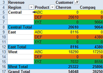
- Format all cells for one product.
If you have multiple column fields, you can select various columns by hovering near the top of the label for a column.
Gotcha: This feature can be turned off. To ensure that it's not turned off, enable the Enable Selection setting under the Select dropdown on the Options tab.