Excel: Apply Conditional Formatting to a Pivot Table

Problem: The new conditional formatting options in Excel are amazing, but they require special care in pivot tables. If you include the grand total row, it will get the largest data bars, and the detail cells have relatively meaningless bars.

Strategy: You can use the Manage Rules dialog to assign conditional formatting to only certain cells. You can initially create the "œwrong" formatting and then edit it to refer to only the selected cells. For example, follow these steps:

1. Select cells B5:B15. You want the first cell in the selection to be the correct type of cell. In this case, it is a value for a product.
2. Select Home, Conditional Formatting, Data Bars, Solid Fill, Red. Excel applies data bars, but the region totals are getting the largest bars.

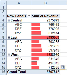
1. Cells B8 & B12 artificially get the largest data bars.
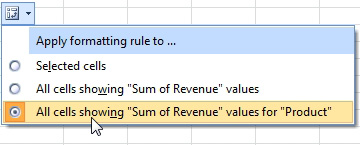
   3. In Excel 2010, open the pivot options dropdown at the bottom right corner of the pivot table. Choose to apply the formatting rule to only cells for revenue and product.

   

2. In Excel 2010, a dropdown appears in the grid.

   

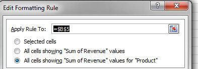
3. Go to the Edit Rules dialog in Excel 2007.

   Results: the data bars are applied only to the detail product rows.

   

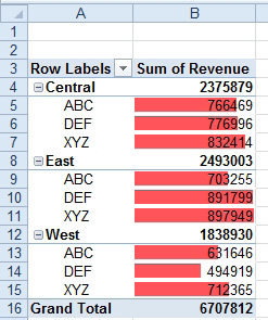
4. The data bars are applied only to like cells.

   Additional Details: Similar settings are available for icon sets and color scales.