Excel: Unapply a Filter Using DAX

Contrast SUMIFS and CALCULATE.

• With SUMIFS, you go through a data set, finding rows that match all of the criteria.
• With Calculate, you go through a data set, calculating values that match the filters in calculate. BUT...you also have an external outside force that is forcing other filters to be applied. Those filters might be coming from the slicers or even from the row and column labels. When PowerPivot goes about calculating cell F4 in the figure above, it has to respect the weekday=Saturday in the calculate function, but it also has to respect Month=Jan caused by the row label in D4 and Year=2016 caused by the slicer.

Ready for something amazing? The filters in calculate have the power to tell the external outside force to not apply a certain filter. If that formula up in F4 used a filter of Month="Feb", the filter in the Calculate formula would override the filter from the row label in D4. Let me show you an example.

Consider this figure.

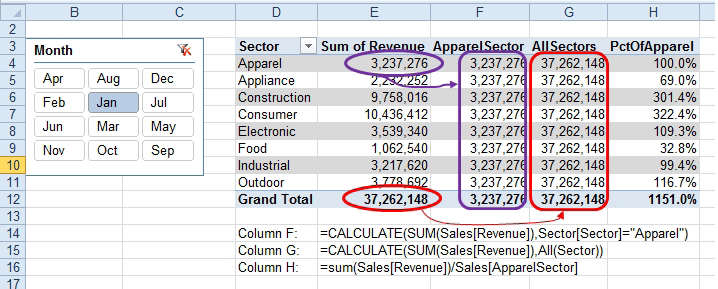
1. These DAX Measures unapply a filter.
   • Column E, Sum of Revenue is a regular old field where I took the Revenue field from the field list and put it in the values drop zone. Column E respects the filters in the slicer and the filters of the row labels in column D.
   • Column F is a DAX Measure where I used CALCULATE to override the filter on sector. No matter what label is over in column D, the DAX measure in column F will filter sector to Apparel. Column F still continues to respect the month slicer, though. The formula for the measure in F is =CALCULATE(SUM(Sales[Revenue]),Sector[Sector]="Apparel")
   • Column G is a DAX Measure where I wiped out the Sector filter by using ALL. Every row in column G is going to show the total for all sectors, even though the row label in D5 says that this row is for Appliance. The formula for the measure in G is =CALCULATE(SUM(Sales[Revenue]),All(Sector)). Note that this formula still respects the filter applied in the month slicer.
   • Column H is the actual useful field. It takes the revenue for this sector and divides it by the revenue for the Apparel sector. The formula here re-uses the existing DAX measure from column F: =sum(Sales[Revenue])/Sales[ApparelSector]. Of course, this formula still respects the month filter applied from the slicer.

   As you change the filters other than sector, all of the formulas update. Here is the same pivot table filtered to June, July, and August.

   

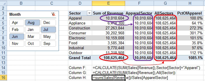
2. Change any filters other than Sector to recalculate.