Problem: I need to do a lookup where I find the product ID down the left side and the month from the top row. I need to return the intersection of that row and column.
Strategy: You can use a MATCH to find the row, a second MATCH to find the column, and then an INDEX to return the correct value.
In this example, the person using the spreadsheet uses the Validation dropdowns in J2 and J3 to select a product and month.
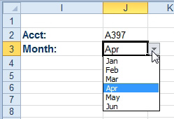
- Select a product and month.
The lookup table has products in column A and months in row 1.
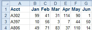
- Find product A397 and Apr.
Your first formula will use MATCH to find the row within the table. Use =MATCH(J2,$A$2:$A$20,0). This is the same type of MATCH described in the previous three topics. The answer of 2 indicates that A397 is found in the second row of the lookup table.
The second formula will use MATCH to find the column within B1:G1. This means that MATCH can go both ways and essentially do an HLOOKUP. Use =MATCH(J3,B1:G1,0). The result of 4 indicates that Apr is in the fourth column of the lookup table.
Finally, use the INDEX function to return the value from row specified by the MATCH in J5 and from the column specified in J6. Use this formula: =INDEX(B2:G20,J5,J6).
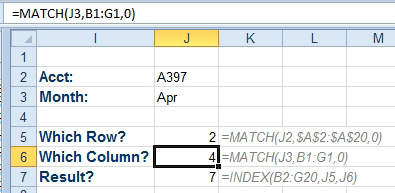
- The MATCH in J6 is like an HLOOKUP.