
Problem: A pivot table organizes data alphabetically by default. I want to produce a report that is sorted high to low by revenue.
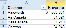
- Reports are normally sorted alphabetically.
Strategy: Each pivot table field offers a sort option. To access the sort options for a field, follow these steps:
- Open the Customer field dropdown in cell A3. Gotcha: Depending on the layout, this field might be called Row Labels instead of Customer.
- Choose More Sort Options.
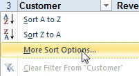
- Choose More Sort Options.
- Excel displays the Sort (Customer) dialog. Initially, the sort is set to Manual. This option lets you re-sequence items by dragging or retyping as discussed in the previous topic. Choose Descending. Open the dropdown under Descending and choose Revenue.
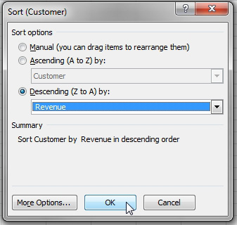
- Choose descending by Revenue.
Results: The report will be sequenced with the largest customers at the top.
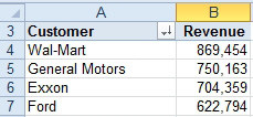
- Largest customers at the top.
Further, as you continue to pivot this report, Excel will remember that customers should always be sorted based on descending revenue. In this figure, product is added as an outermost row field. The report is automatically sorted, this time with Exxon at the top.
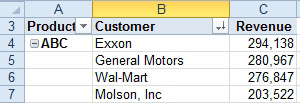
- Customer continues to re-sort after pivoting.
Additional Details: If you use the Compact Form layout with multiple row fields, there is an extra step. When you open Row Labels, you have to choose from a second dropdown to choose which field you want to sort.
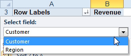
- Extra dropdown in Compact Form layout.
An alternate method for accessing the Sort dialog is to hover over the Customer field in the top of the PivotTable Field List dialog. A dropdown appears. You can choose to sort or filter from this dropdown.