
Problem: Sometime, back in the days of COBOL, a programmer was dealing with the constraints of the physical width of a page. The programmer built a report in which each record actually took up five lines of the report. I want to be able to analyze this data in Excel.
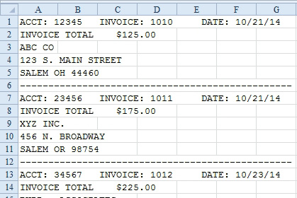
- Transform this frustrating data set.
Strategy: Your goal is to get the data back into one row per record. This process involves adding two new columns, Group and Sequence:
- Add a new row 1. Insert two new columns, A and B. Add the headings Group, Seq, and Text in A1:C1.
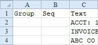
- Add two new columns.
- In column A, assign a group number to each logical record. One way to do this is to check to see if the first four characters of column C are ACCT. If they are, add 1 to the group number. In A2, enter the number 1. In A3, enter the formula =IF(LEFT(C3,4)="ACCT",1+A2,A2). (This is similar to the formula from "Add a Group Number to Each Set of Records That Has a Unique Customer Number".) Copy it down to all the rows. Excel will assign a group number to each logical group of records.
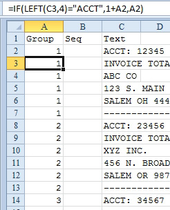
- Use the IF function.
- Design a formula for a sequence number. To do this, in cell B2, enter the formula =IF(A2=A1,B1+1,1). (This formula is like the one from "Number Each Record for a Customer, Starting at 1 for a New Customer") Copy this down. This formula will number each record in the group. It should ensure that all the account numbers are on a Sequence 1 record.
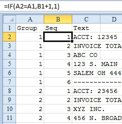
- Formula for sequence number.
- (This step is critical.) Copy the formulas in columns A and B and paste them back, using Home, Paste dropdown, Paste Values to ensure that you can safely sort the data.
- Sort the data by the sequence number in column B. Your data will look like this.
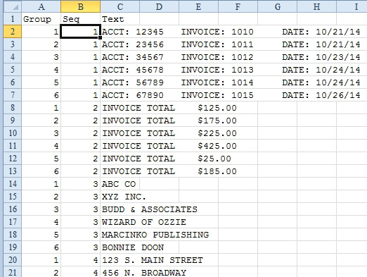
- Sort the data into record types.
You have now managed to intelligently segregate the data so that all similar records are together. The contiguous range C2:C7 contains all the first rows from each record. Each of the line 1 records has three fields that really should be parsed into three separate columns. You can easily do this parsing with the Text to Columns Wizard.
- Select cells C2:C7. Select Data, Text to Columns to open the Convert Text to Columns Wizard. Select Fixed Width. Click Next.
- Excel should properly guess where your columns are. Click Next.
- Choose the heading for each column and define a data format. You don't really need the word ACCT each time, so choose to skip the first, third, and fifth fields. Make the sixth field a date. When your information looks as shown below, click Finish. You will have data in three columns of Group 1.
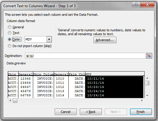
- In Step 3, skip columns 1, 3, and 5. Choose Date for col. 6.
- Change the heading in C1 to Acct, the heading in D1 to Inv, and the heading in E1 to Date.
- Select and cut A8:C13 and paste into F2.
- Delete Group & Seq from F & G.
- Add the heading of Inv $ to F1.
- Select F2:F6 and choose Data, Text to Columns. In Step 1 of the wizard, select Fixed Width and click Next. In Step 2 of the wizard, Excel offers to split your data into three fields. There is no need to have one column for the word Invoice and another column for the word Total.
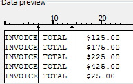
- Excel suggests an extra column.
- Double-click the line between Invoice and Total to delete it.
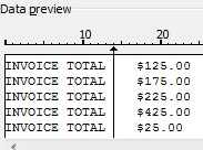
- Double-click the extra line to delete it.
- In Step 3 of the wizard, choose to skip the field that contains Invoice Total. Click Finish.
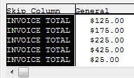
- Skip the field label.
- Records for Groups 3 through 5 only have a single field without a heading. Copy C14:C19 to G2. Add a heading of Company.
- Copy Group 4's column C cells to H2. Add a heading of Address.
- Copy Group 5's column C cells to I2. Add a heading of City ST Zip.
- Because the Group 6 records have no data-they are just dashed lines-delete these rows.
You now have all the fields, one line per record.
- Delete the columns extra columns A& B.
Results: You now have a sortable, filterable, and reportable version of the original data set. Each record consists of one row in Excel.
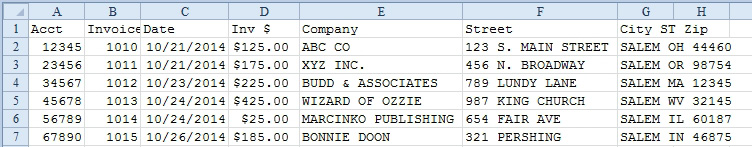
- You can now sort and analyze this data.