Excel: Data Model

Problem: I have a lot of rows in a data table and then some lookup tables. Is there a faster way to create a report than building a bunch of VLOOKUP formulas?

Strategy: Excel 2013 adds a pivot table feature called the Data Model. This will solve the problem. This will work in all versions of Excel 2013, whether you have the Power Pivot tab installed or not.

The process works much better if you declare all of your data sets to be Ctrl+T tables first.

1. Select one cell in your main data set and press Ctrl+T. Confirm that the data has headers and click OK.
2. In the Table Tools Design tab, you will see a name for the table. Type a meaningful name, something like Data.
3. Select one cell in your lookup data. Ctrl+T. OK. Rename this table Sectors.
4. Go back to the original data. Select one cell. Insert, Pivot Table.
5. In the Create Pivot Table dialog, check the box for Add This Data to the Data Model. Click OK.

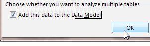
1. Checking this box opens a wide variety of new options.

   It seems like a really innocuous box, but by checking that box in Excel 2013, you are loading the data into the Power Pivot data model that is hidden behind Excel 2013. If this is the first time you've used the Data Model in this Excel session, you might notice a few-second delay before you get to the Pivot Table Field list.

   At this point, everything feels like a regular pivot table with one small change. You will notice a line at the top of the Pivot Table Field List offering ACTIVE | ALL.

   

2. Before you move on to All, create a relationship.
   6. Go to the Analyze tab in the ribbon. Choose Relationships. Click New...
   7. There are four fields to fill out in the Create Relationship dialog. Start from your Data table and choose the key field used to link to the lookup table. For the Related table, choose the lookup table and the key field. Click OK.

   

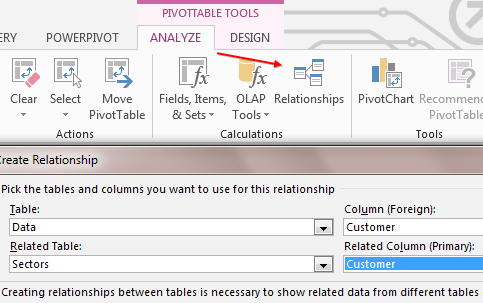
3. This is far easier than a VLOOKUP.
   8. You can now go to the ALL section of the Pivot Table Fields.
   9. You can now expand each table and choose fields from that table.

   

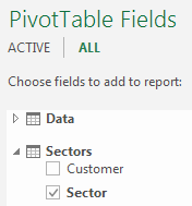
4. Choose fields from any table.

   The result is a pivot table with fields from Sheet1 and Sheet2.

   

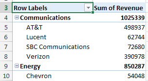
   Joining two tables in a pivot table is an amazing improvement. Although Excel calls this the Data Model, it is really the Power Pivot Engine. Even if you don't have two tables to join, there are some interesting reasons to run the data through the Data Model. See January Actuals and February Plan later in this chapter.