Excel: Create a Flattened Pivot Table for Reuse

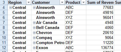
Problem: Why would they put three different kinds of information in column A? Doesn't this make pivot tables as silly as the person who created the bad data set back in "œAdd a Customer Number to Each Detail Record"?

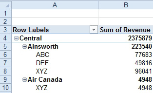
1. Microsoft is mixing 3 fields in one column.

   My goal is to use the pivot table to make a summary, then convert to values for use as a new data set. Having three different fields in column A is really bad form.

   Note: I've met one person who likes compact view. He has 15 fields in the Row Area of his report. Compact layout allows that report to fit on a screen.

   Strategy: It is very annoying that Microsoft made this new view be the default. Luckily, it is only a few clicks to go back to the proper view.

   1. Select one cell in the pivot table.
   2. Choose the Design tab of the ribbon.
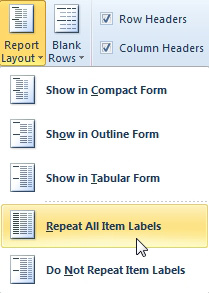
   3. Open the Report Layout dropdown.
   4. Change from Compact Form to Tabular Form.
   5. If you have Excel 2010, open the Report Layout dropdown again and choose Repeat All Item Labels.

   

2. New in Excel 2010, eliminate blanks in the row area.
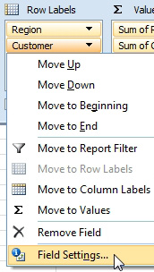
   6. For each field in the Row Area except the last field, open the dropdown in the Row Area dropdown and choose Field Settings.

   

3. Access field settings for all but the final row field.
   7. In the Field Settings dialog, choose None for Subtotals.

   

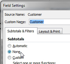
4. Turn off the subtotals for the outer row fields.
   8. On the Design tab, open the Grand Total dropdown and choose Off for Rows and Columns.

   The result is a flattened pivot table, perfect for re-use as a new consolidated data set. Copy the pivot table and paste as values to a new worksheet.

   

5. Copy and Paste Values this pivot table for re-use.