
The example in "Can I Save Formatting in a Template?" on page 369 used GetPivotData to show Actual for some months and Plan for other months.
Good news: Excel 2010 offers a new feature called named sets that finally allows you to create asymmetric reports.
Bad news: Named sets work only with OLAP pivot tables for this release, so you cannot use them with regular pivot tables.
Good news: If you take your regular Excel data through PowerPivot, the data becomes an OLAP pivot table, and therefore you can use named sets.
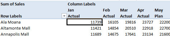
To recap the problem, you want to show Actuals for January through April and Plan for the remaining months:
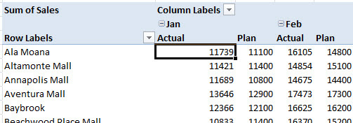
- Show Actuals for some months and Plan for other months.
In the PivotTable Tools Option tab, choose Fields, Items, Sets and choose Create Set Based on Column Items.
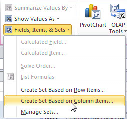
- Create a named set.
Excel shows you a dialog with a new row for every column in your pivot table. Highlight a column and click Delete Row to remove it from the pivot table.
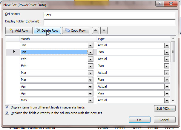
- You can delete specific columns from the set.
You eventually end up with a list of only the desired columns.
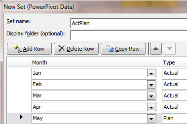
- Keep deleting columns until only the desired items are left.
The resulting pivot table is shown below. It is amazing how hard this is in regular pivot tables, but certainly possible with PowerPivot datasets.
- The named set leaves an asymmetric pivot table.