
Problem: I need to total only the visible cells in a filtered data set.
Strategy: You can use the AutoSum icon after applying a filter. Normally, the AutoSum icon inserts a SUM function. When you apply a filter and then use AutoSum, Excel will insert a SUBTOTAL function instead. This function will ignore rows hidden by the Filter command. Follow these steps:
- Choose a cell in your data set. Select Data, Filter.
- Apply a filter to at least one column. Open the Customer dropdown and choose one customer.
- Select the first visible cells beneath your numeric columns. Below, the last visible row is 539, but the next blank cell is in row 568.
- Click the AutoSum icon and press Enter. Excel inserts a SUBTOTAL function that uses the correct syntax to skip rows hidden by the filter.
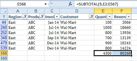
- Excel inserts the SUBTOTAL function.
When you choose a different selections from the filter dropdown, the SUBTOTAL function will show the total for those visible.
Additional Details: During a seminar for the Fort Wayne IIA, someone added a great suggestion to this topic. Insert two blank rows at the top. Cut the formulas from the total row and paste to row 1. Now, even if the filtered rows are more than will fit on a screen, you always have the filtered totals at the top.