Excel: Format Every Other Row in Green

Problem: Got any cool uses for MOD? Got any old-school methods for applying the greenbar format that was in the Excel 2003 AutoFormat dropdown?

Strategy: This topic is about an out-of-the-box method for using MOD to apply a format. If the only goal was to apply alternate-row shading, you could use any of these methods:

• Alt+O+A and choose the Excel 2003 format.
• Ctrl+T, choose Banded Rows and any format.
• Leave row 2 unformatted. Fill row 3 with green. Select row 2 & row 3. Use the fill handle to drag to the bottom of the data set. Open the Paste Options menu and choose Fill Formatting Only.

However, this topic is going to use math to do the formatting.

Consider the ROW function. =ROW(A2) will return 2 because A2 is in the second row of the worksheet. Here is a big range of ROW functions.

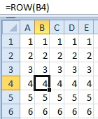
1. The ROW function tells you the row number.

   Now, imagine taking all of those row numbers and dividing by 2. Throw away any integer result, but keep the remainder. This is a strange thought. All of the even number rows will not have a remainder at all. For the odd number rows, say that you take seven divided by 2. You get 3 with a remainder of 1. Throw out the 3 and keep only the remainder. The MOD function will give you only the remainder. =MOD(ROW(A7),2) will return a 1 because 7 divided by 2 has a remainder of 1. The next figure shows the MOD formula for several rows. Notice that you get stripes of 0's and 1's.

   

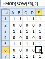
2. MOD of the ROW, 2 will return stripes.

   So, how do you use this formula to add a green stripe in every other row? You do it with old-school conditional formatting. Follow these steps.

   1. Select your range of data. Perhaps it is A2:G900.
   2. Make a note of which cell is the active cell. This is the cell address that is shown in the Name box, to the left of the formula bar. You will need this cell address in step 4.
   3. Select Home, Conditional Formatting, New Rule.
   4. There are six types of rules listed in the top of the New Formatting Rule dialog. Choose the last type, called Use A Formula To Determine Which Rows To Format. When you choose this type, a formula bar appears in the bottom of the dialog. It is called Format Values Where This Formula is True.
   5. Click in that formula box. Type a formula similar to this formula, but use the cell address from step 2 instead of A2. =MOD(ROW(A2),2)=1.
   6. Click the Format"¦ button.
   7. On the Fill tab, choose a fill color. Click OK.

   

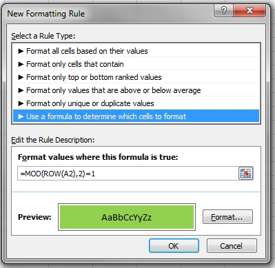
3. Your dialog should look like this one.
   8. Click OK to apply the rule.

   The range will be filled with an every-other row format.

   

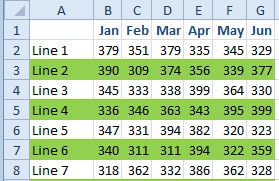
4. Greenbar format.

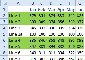
   The cool part is that if you delete a row or insert a row, the MOD(ROW(),2) formulas will recalculate and the shading will redraw. In the figure below, Line 3a is now green and Line 4 is white.

   

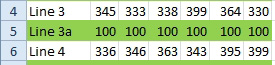
5. The formatting recalcs after inserting rows.

   Additional Details: With a little math reasoning, you can change the format pattern. What if you wanted the even rows to be formatted? Change the formula to =MOD(ROW(A2),2)=0. If you wanted two rows of green followed by two rows of white, use =MOD(ROW(A2),4)>1.

   

6. Divide the row by 4. If the remainder isn't 0 or 1, use green.